图像的基本操作

• 1.读取图像
• • 1.1代码实现
  • 1.2两者的差异
• 2.创建图像缩略图
• • 2.1代码实现
  • 2.2两者的差异
• 3.绘制图像的轮廓与直方图
• • 3.1代码实现
  • 3.2运行结果
• 4.实现图像的灰度变换、直方图均衡化
• • 4.1代码实现
  • 4.2运行结果
• 5.实现图像的不同高斯模糊、计算导数
• • 5.1代码实现
  • 5.2运行结果
• 6.形态学计数（计算圆形个数等）、去噪
• • 6.1代码实现
  • 6.2运行结果
• 7.小结

1.读取图像

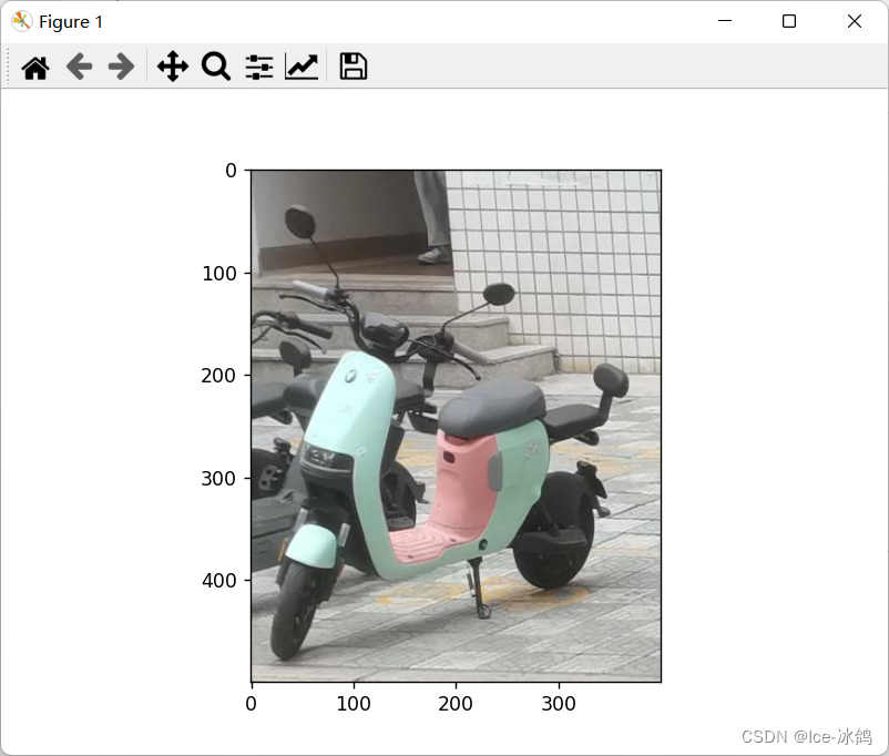
本实验分别使用PIL库和OpenCV库读取图像并实现可视化，并对比OpenCV读取和PIL读取的差异。

1.1代码实现

# Using PIL library
from PIL import Image
import matplotlib.pyplot as pltimg_pil = Image.open('001.jpg')
plt.imshow(img_pil)
plt.show()# Using OpenCV library
import cv2img_cv = cv2.imread('001.jpg')
cv2.imshow('image', img_cv)
cv2.waitKey(0)
cv2.destroyAllWindows()

先是PIL库的可视化：

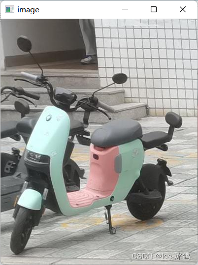
这是OpenCV库的可视化：

1.2两者的差异

• 颜色空间
  PIL库默认使用RGB颜色空间读取图像，而OpenCV库默认使用BGR颜色空间读取图像。这意味着，如果我们使用OpenCV库读取图像并使用PIL库显示图像，图像的颜色可能会有所不同。
• 数据类型
  PIL库使用的图像数据类型为PIL.Image，而OpenCV库使用的图像数据类型为NumPy数组。这意味着，如果我们想要在两个库之间传递图像数据，需要进行数据类型的转换。
• 图像大小
  PIL库读取图像时会将图像缩放到适合显示的大小，而OpenCV库读取图像时不会自动缩放图像。因此，在使用OpenCV库显示图像时，我们需要手动调整图像的大小。

2.创建图像缩略图

2.1代码实现

# Using OpenCV library
import cv2img_cv = cv2.imread('001.jpg')
img_cv = cv2.resize(img_cv, (300, 300)) # resize image
cv2.imshow('image', img_cv)
cv2.waitKey(0)
cv2.destroyAllWindows()# create thumbnail
img_cv_thumbnail = cv2.imread('001.jpg')
img_cv_thumbnail = cv2.resize(img_cv_thumbnail, (100, 100)) # resize image
cv2.imshow('thumbnail', img_cv_thumbnail)
cv2.waitKey(0)
cv2.destroyAllWindows()

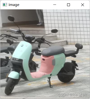
先是resize

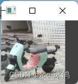
然后是thumbnail函数

2.2两者的差异

thumbnail()和resize()都是PIL库中的图像处理函数，可以用来改变图像的尺寸。它们的不同在于thumbnail()会保持图像的宽高比例，同时尽可能的缩小图像以适应给定的大小。而resize()则可以通过指定目标图像的宽度和高度来改变图像的大小，它不会保持图像的宽高比例。

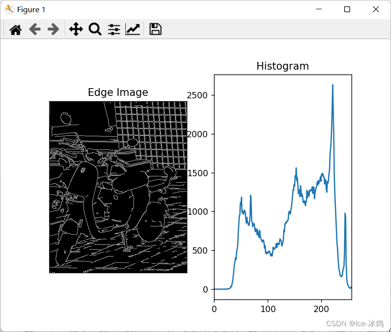
3.绘制图像的轮廓与直方图

3.1代码实现

import cv2
import numpy as np
from matplotlib import pyplot as plt# 读取图像
img = cv2.imread('001.jpg', 0)# 绘制轮廓
edges = cv2.Canny(img, 100, 200)
plt.subplot(121), plt.imshow(edges, cmap='gray')
plt.title('Edge Image'), plt.xticks([]), plt.yticks([])# 绘制直方图
hist = cv2.calcHist([img], [0], None, [256], [0, 256])
plt.subplot(122), plt.plot(hist)
plt.title('Histogram'), plt.xlim([0, 256])plt.show()

3.2运行结果

这是该图片的轮廓和直方图：

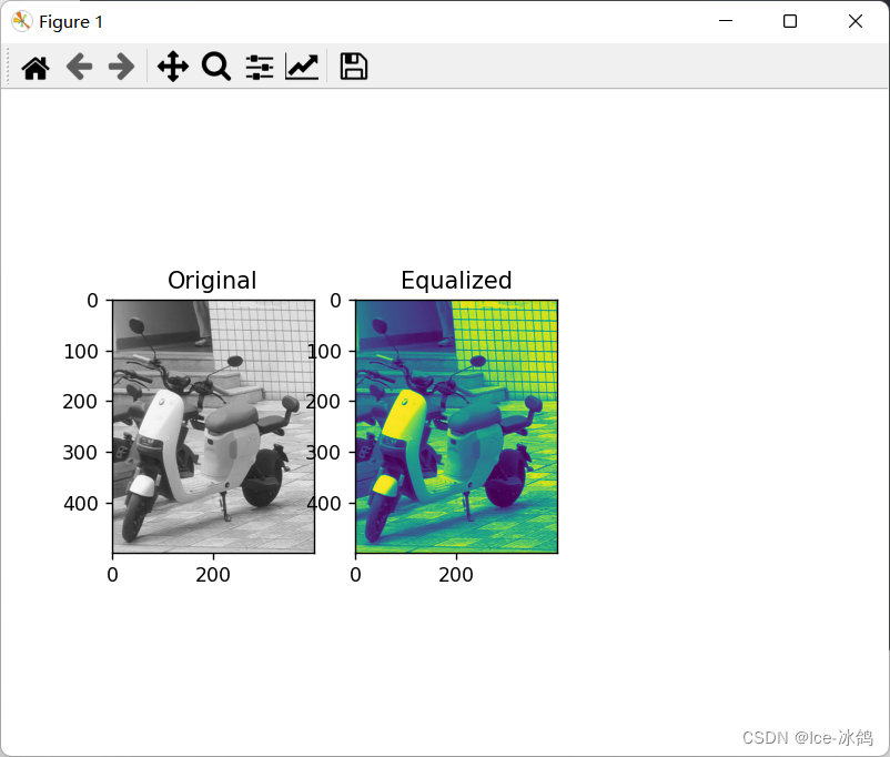
4.实现图像的灰度变换、直方图均衡化

4.1代码实现

import cv2
import numpy as np
import matplotlib.pyplot as plt# 读取图像
img = cv2.imread('001.jpg', cv2.IMREAD_GRAYSCALE)# 灰度变换
img_gray = cv2.cvtColor(img, cv2.COLOR_GRAY2BGR)# 直方图均衡化
img_eq = cv2.equalizeHist(img)# 显示图像
plt.subplot(1, 3, 1)
plt.imshow(img_gray)
plt.title('Original')plt.subplot(1, 3, 2)
plt.imshow(img_eq)
plt.title('Equalized')plt.show()

4.2运行结果

以下是运行结果：

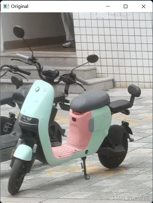
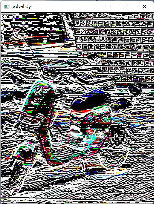
5.实现图像的不同高斯模糊、计算导数

5.1代码实现

import cv2
import numpy as np# Load image
img = cv2.imread('001.jpg')# Gaussian blur with kernel size 3x3
blur_3x3 = cv2.GaussianBlur(img, (3, 3), 0)# Gaussian blur with kernel size 5x5
blur_5x5 = cv2.GaussianBlur(img, (5, 5), 0)# Calculate derivatives using Sobel operator
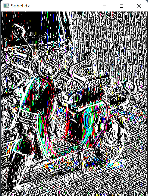
dx = cv2.Sobel(img, cv2.CV_64F, 1, 0, ksize=3)
dy = cv2.Sobel(img, cv2.CV_64F, 0, 1, ksize=3)# Display results
cv2.imshow('Original', img)
cv2.imshow('3x3 Gaussian Blur', blur_3x3)
cv2.imshow('5x5 Gaussian Blur', blur_5x5)
cv2.imshow('Sobel dx', dx)
cv2.imshow('Sobel dy', dy)
cv2.waitKey(0)
cv2.destroyAllWindows()

5.2运行结果

原始图片

3×3高斯模糊

5×5高斯模糊

Sobel对x的梯度

Sobel对y的梯度

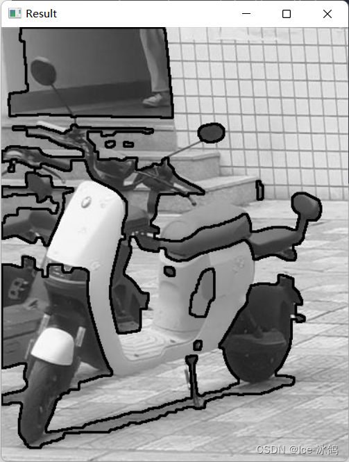
6.形态学计数（计算圆形个数等）、去噪

6.1代码实现

import cv2
import numpy as np# Load image
img = cv2.imread('001.jpg', cv2.IMREAD_GRAYSCALE)# Apply Gaussian blur to remove noise
blur = cv2.GaussianBlur(img, (5, 5), 0)# Apply thresholding to convert image to binary
_, thresh = cv2.threshold(blur, 0, 255, cv2.THRESH_BINARY_INV+cv2.THRESH_OTSU)# Apply morphological operations to remove noise and fill holes
kernel = np.ones((3,3), np.uint8)
opening = cv2.morphologyEx(thresh, cv2.MORPH_OPEN, kernel, iterations=2)
closing = cv2.morphologyEx(opening, cv2.MORPH_CLOSE, kernel, iterations=2)# Find contours and draw them on the original image
contours, hierarchy = cv2.findContours(closing, cv2.RETR_EXTERNAL, cv2.CHAIN_APPROX_SIMPLE)
cv2.drawContours(img, contours, -1, (0, 0, 255), 2)# Count the number of circles
circles = cv2.HoughCircles(closing, cv2.HOUGH_GRADIENT, 1, 20, param1=50, param2=30, minRadius=0, maxRadius=0)
if circles is not None:circles = np.round(circles[0, :]).astype("int")print("Number of circles:", len(circles))
else:print("No circles found")# Display the result
cv2.imshow('Result', img)
cv2.waitKey(0)
cv2.destroyAllWindows()

6.2运行结果

高斯去噪后在原图上画出轮廓

命令行输出

从上面的轮廓图就可以看出本图没有圆形轮廓，所以计数应该是0。

7.小结

本次实验主要使用了OpenCV库对图像进行处理，包括读取、可视化、缩略、变换、绘制轮廓和直方图、灰度变换、直方图均衡化、高斯模糊、计算导数、形态学计数和去噪等应用。OpenCV库适合用于计算机视觉应用程序，可应用于图像分析和处理。